Kaggle - Heart Disease Dataset (1)에서 우리가 데이터 셋을 분석 해봤었습니다. 다시 한번 확인을 해볼까요?
| 1. age | 나이 (int) |
| 2. sex | 성별 (1, 0 / int) |
| 3. chest pain type (4 values) | 가슴 통증 타입 (0 ~ 3 / int) |
| 4. resting blood pressure | 혈압 |
| 5. serum cholestoral in mg/dl | 혈청 콜레스테롤 |
| 6. fasting blood sugar > 120 mg/dl | 공복 혈당 |
| 7. resting electrocardiographic results | 심전도 |
| 8. maximum heart rate achieved | 최대 심장박동 수 |
| 9. exercise induced angina | 운동 유도 협심증 (이게 뭐죠?) |
| 10. oldpeak = ST depression induced by exercise relative to rest | 노약 =운동에 의해 유발되는 St 우울증 (이건 또 뭐죠?) |
| 11. the slope of the peak exercise ST segment | ST 세그먼트의 기울기 |
| 12. number of major vessels (0-3) colored by flourosopy | 혈관의수 |
| 13. thal : 3 = normal; 6 = fixed defect; 7 = reversable defect | 뭔지 모르겠네요 |
이렇게 위 데이터 셋이 구성된 것을 확인했었습니다. 이제 저희는 one-hot-encoding과 model을 만들어서 logisitc regression(로지스틱 회귀)를 적용해보도록 하겠습니다.
우선 one-hot-encoding을 위해 dummy variables를 만들어 보도록 하겠습니다.
a = pd.get_dummies(data['cp'], prefix = "cp")
b = pd.get_dummies(data['thal'], prefix = "thal")
c = pd.get_dummies(data['slope'], prefix = "slope")
여기서 'cp', 'thal', 'slope' 데이터는 categorical variables라서 one-hot-encoding을 적용했습니다. categorical data는 제가 쓴 Machine / Deep Learning 용어 설명에서 썼듯이 여러 Categories들 중 하나의 이름에 데이터를 분류할 때 사용합니다. (예: 청팀 : 0, 백팀 : 1, 홍팀 : 2)
frames = [data, a, b, c]
data = pd.concat(frames, axis = 1)
data.head()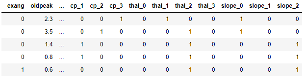
dummies로 만들었으니 하나로 합쳤습니다. 근데, dummies로 만들어지기 전 데이터는 필요없는 데이터니 버리도록 해볼까요? drop으로 버리도록 해봅시다.
data = data.drop(columns = ['cp', 'thal', 'slope'])One-hot-encoding을 마쳤으니 이제 진짜 Logistic Regression을 위한 모델을 세워보도록 합시다.
저희는 sklearn libarary 또는 직접 함수를 작성할 수 있습니다. 한번 둘 다 해보도록 하겠습니다. 첫번째로 함수를 직접 작성해보고 후에 sklearn library를 사용해보도록 합시다.
y = df.target.values
x_data = data.drop(['target'], axis = 1)
Normalize Data (데이터 정규화) - 데이터 정규화란 관계형 데이터베이스의 설계에서 중복을 최소화하게 데이터를 구조화하는 프로세스입니다. 중복성 및 종속성을 제거하고 데이터베이스 변경시 이상현상을 제거해줍니다.
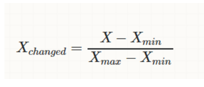
# Normalize
x = (x_data - np.min(x_data)) / (np.max(x_data) - np.min(x_data)).values
Normalize를 했으면 우리의 데이터에서 80%는 train 데이터 20%는 test data로 나누도록 합시다.
x_train, x_test, y_train, y_test = train_test_split(x, y, test_size = 0.2, random_state = 0)# transpose matrices
x_train = x_train.T
y_train = y_train.T
x_test = x_test.T
y_test = y_test.T이제 가중치를 0.01로 하고 편향을 0.0으로 설정을하고 함수를 짜봅시다.
# initialize
def innitialize(dimension):
	weight = np.full((dimension, 1), 0.01)
    bias = 0.0
    return weight, bias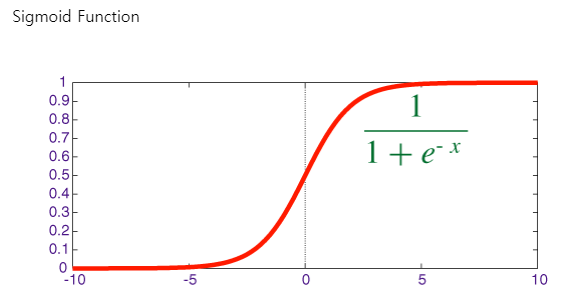
시그모이드 함수는 위의 그림과 같습니다. 얘도 함수로 표현해보도록 하죠
def sigmoid(z):
	y_head = 1/(1 + np.exp(-z))
    return y_head
이제 순전파/역전파 함수, Cost Function, Gradient Descent 함수를 짜보겠습니다. 그 전에 얘들이 어떤 애들인지 얘기를 하고 넘어가도록 하겠습니다.
순전파부터 얘기를 하겠습니다.
순전파 함수는 간단하게 말해서 뉴럴 네트워크의 그래프를 계산하기 위해서 입력층부터 시작해서 출력층까지 중간 변수들을 순서대로 계산하고 저장하는 함수입니다.
역전파 함수는 중간 변수와 파라미터에 대한 Gradient(변화)를 반대 방향으로 계산하고 저장하는 함수입니다.
Input에서 Output으로 가중치를 업데이트하면서 활성화 함수를 통해서 결과값을 가져오는 것이 순전파라고 말합니다. 하지만 임의로 한 번 순전파를 거쳤다고 출력 값이 정확하지는 않을 것입니다. 임의로 설정한 가중치 값이 input에 의해서 한 번 업데이트 되지만 문제가 발생할 수 있기 때문입니다.
역전파 방법은 결과 값을 통해서 다시 역으로 input 방향으로 오차를 보내며 가중치를 재 어데이트 하는 것입니다. 물론 결과에 영향을 많이 미친 노드에 더 많은 오차를 돌려줄 것입니다.
이제 Cost Function을 얘기해봅시다.
cost function은 학습이 완료된 후의 평균 에러를 다루는 함수입니다. 즉 loss function의 합, entire data set을 다루는 함수입니다. 더 자세한 것은 제가 쓴 용어 설명을 참조하시길 바랍니다.
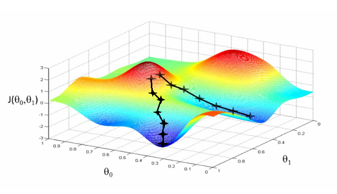
Gradient Descent 함수는 경사하강법입니다.
경사하강법은 오차함수의 낮은 지점을 찾아가는 최적화 방법입니다. 즉, 가중치를 수정해가면서 오차가 낮은 쪽의 방향을 찾기 위한 것으로 오차함수를 현재 위치에서 미분을 하면 됩니다.
하지만 최저점이 많을 경우 우리가 원하는 진짜 최저점을 찾기 어려울 수 잇습니다. 이런 경우엔 가중치(weight)의 초기 값을 다르게 주면서 경사하강법을 활용하면 됩니다.
설명을 마쳤으니 함수로 표현해보도록 하겠습니다.
def forwardBackward(weight, bias, x_train, y_train):
	# Forward

    y_head = sigmoid(np.dot(weight.T, x_train) + bias)
    loss = -(y_train * np.log(y_head) + (1-y_train) * np.log(1-y_head))
    cost = np.sum(loss) / x_train.shape[1]

    # Backward
    derivative_weight = np.dot(x_train, ((y_head-y_train).T)) / x_train.shape[1]
    derivative_bias = np.sum(y_head-y_train) / x_train.shape[1]
    gradients = {"Derivative Weight" : derivative_weight, "Derivative Bias" : derivative_bias}

    return cost, gradients
def update(weight, bias, x_train, y_train, learningRate, iteration):
costList = []
index = []
# for each iteration, update weight and bias values
for i in range(iteration):
cost, gradients = forwardBackward(weight, bias, x_train, y_train)
weight = weight - learningRate * gradients["Derivative Weight"]
bias = bias - learningRate * gradients["Derivative Bias"]
costList.append(cost)
index.append(i)
parameters = {"weight" : weight, "bias" : bias}
print("iteration:", iteration)
print("cost:", cost)
plt.plot(index, costList)
plt.xlabel("Number of Iteration")
plt.ylabel("Cost")
plt.show()
return parameters, gradientsdef predict(weight, bias, x_test):
z = np.dot(weight.T, x_test) + bias
y_head = sigmoid(z)
y_prediction = np.zeros((1, x_test.shape[1]))
for i in range(y_head.shape[1]):
if y_head[0, i] <= 0.5:
y_prediction[0, i] = 0
else:
y_prediction[0, i] = 1
return y_predictiondef logistic_regression(x_train, y_train, x_test, y_test, learningRate, iteration):
dimension = x_train.shape[0]
weight, bias = initialize(dimension)
parameters, gradients = update(weight, bias, x_train, y_train, learningRate, iteration)
y_prediction = predict(parameters["weight"], parameters["bias"], x_test)
print("Manuel Test Accuracy: {:.2f}%".format((100 - np.mean(np.abs(y_prediction - y_test)) * 100)/100*100))logistic_regression(x_train, y_train, x_test, y_test, 1, 100)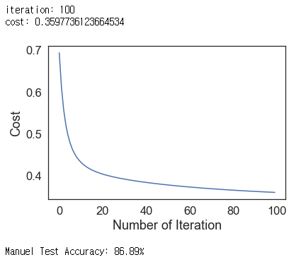
아휴 직접 Logistic Regression을 구현하느라 힘들었습니다. 하지만 우리의 python에는 sklearn이라는 훌륭한 라이브러리가 있습니다. 간단하게 라이브러리를 써서 구해보도록 하겠습니다.
lr = LogisticRegression()
lr.fit(x_train.T, y_train.T)
print("Test Accuracy {:.2f}%".format(lr.score(x_test.T, y_test.T) * 100))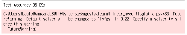
끝입니다.
네 끝이에요.
간단하죠?
한 김에 여러 알고리즘을 사용해서 정확도를 살펴봅시다.
이번에 적용할 알고리즘은 K-Nearest Neighbour (KNN) Classification 입니다.
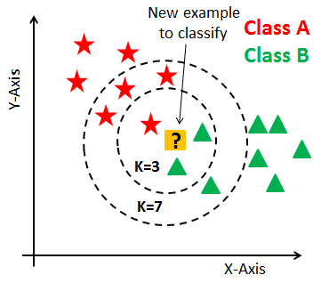
# KNN Model
from sklearn.neighbors import KNeighborsClassifier
knn = KNeighborsClassifier(n_neighbors = 2) # n_neighbors means k
knn.fit(x_train.T, y_train.T)
prediction = knn.predict(x_test.T)

print("{} NN Score: {:.2f}%".format(2, knn.score(x_test.T, y_test.T)*100))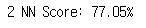
# try to find best k value
scoreList = []
for i in range(1, 20):
    knn2 = KNeighborsClassifier(n_neighbors = i) # n_neighbors means k
    knn2.fit(x_train.T, y_train.T)
    scoreList.append(knn2.score(x_test.T, y_test.T))

plt.plot(range(1, 20), scoreList)
plt.xticks(np.arange(1,20,1))
plt.xlabel("K value")
plt.ylabel("Score")
plt.show()

print("Maximum KNN Score is {:.2f}%".format((max(scoreList))*100))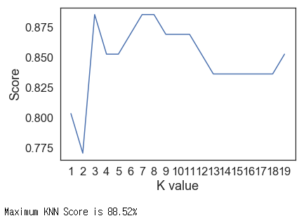
K가 언제일 때 정확도가 최대인지를 구해봤습니다. 우리가 임의로 한 2일 때가 가장 낮았네요. 역시 인생에서 감으로 찍는건 항상 옳은 법이 없는 법이죠. 항상 철저하게 고려해봅시다.
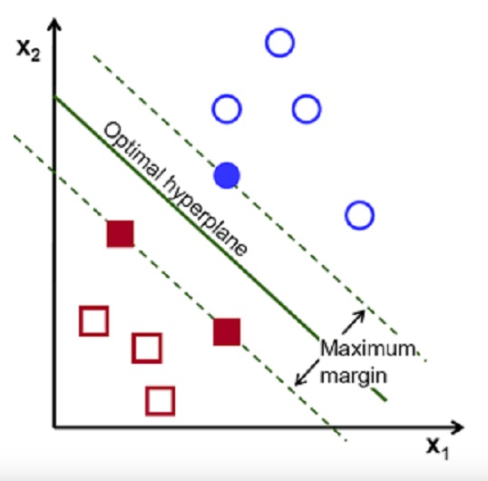
그래서 우리는 Support Vector Machine Algorithm (SVM)도 사용해볼것입니다.
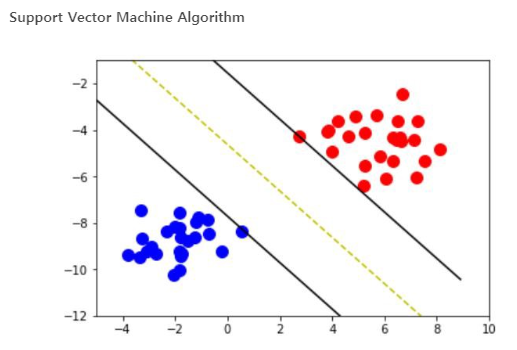
from sklearn.svm import SVCsvm = SVC(random_state = 1)
svm.fit(x_train.T, y_train.T) # 학습시킵시다.print("Test Accuracy of SVM Algorithm: {:.2f}%".format(svm.score(x_test.T, y_test.T)*100))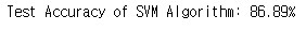
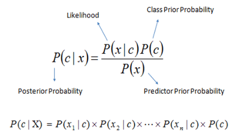
Naive Bayes Algorithm도 써보도록 합시다.
from sklearn.naive_bayes import GaussianNB
nb = GaussianNB()
nb.fit(x_train.T, y_train.T)
print("Accuracy of Naive Bayes: {:.2f}%".format(nb.score(x_test.T, y_test.T)*100))
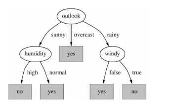
Decision Tree Algorithm도 해봅시다.
from sklearn.tree import DecisionTreeClassifier
dtc = DecisionTreeClassifier()
dtc.fit(x_train.T, y_train.T)
print("Decision Tree Test Accuracy {:.2f}%".format(dtc.score(x_test.T, y_test.T)*100))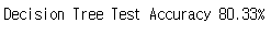
Random Forest Classification도 해봅시다.
# Random Forest Classification
from sklearn.ensemble import RandomForestClassifier
rf = RandomForestClassifier(n_estimators = 1000, random_state = 1)
rf.fit(x_train.T, y_train.T)
print("Random Forest Algorithm Accuracy Score : {:.2f}%".format(rf.score(x_test.T, y_test.T)*100))
우리가 많은 알고리즘을 다뤘는데 이걸 한 눈에 볼 수 있도록 그래프로 그려서 확인 해봅시다.
methods = ["Logistic Regression", "KNN", "SVM", "Naive Bayes", "Decision Tree", "Random Forest"]
accuracy = [86.89, 88.52, 86.89, 86.89, 80.33, 88.52]

sns.set_style("whitegrid")
plt.figure(figsize=(16, 5))
plt.yticks(np.arange(0,100,10))
plt.ylabel("Accuracy %")
plt.xlabel("Algorithms")
sns.barplot(x=methods, y=accuracy)
plt.show()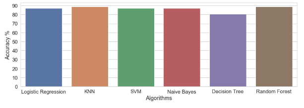
저희의 model이 잘 작동했습니다. Best는 KNN, Random Forest이 최고였습니다 !!
지금까지 Kaggle - Heart Disease Dataset (2) 였습니다. ^_^
'Machine, Deep Learning > Machine, Deep Learning 실습' 카테고리의 다른 글
| 데이터 분석을 위한 삼위일체 (1) (0) | 2019.06.16 |
|---|---|
| Kaggle - 남은 주차공간을 알려주는 AI (1) | 2019.06.15 |
| Kaggle - Heart Disease Dataset (1) (0) | 2019.06.14 |
| Kaggle - MINST 예측 모델 생성 by Keras (2) (2) | 2019.06.10 |
| Kaggle - MINST 예측 모델 생성 by Keras (1) (0) | 2019.06.09 |


